Diffusion models generate images through iterative denoising. They start off from Gaussian noise, then refine it over multiple forward passes. The stochasticity appears via the noise-induced input. Discrete Distribution Networks take a different approach by trying to match the training distribution with a set of discrete candidates. The network outputs a number of discrete candidates at each layer, and generation is done via sequential selection by picking one candidate per layer in a single forward pass. The randomness comes from these discrete choices, not from input noise.

Figure from Yang, 2024

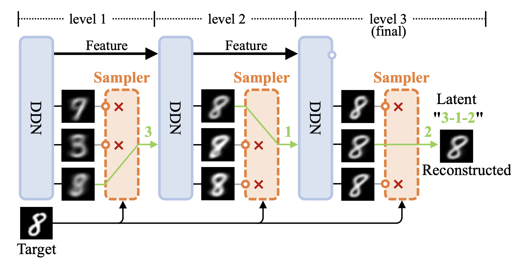
Even though the number of nodes K per layer may be small, stacking multiple DDN layers L leads to $K^L$ possible outputs, creating massive representation capacity. Even modest values (K=64, L=10) yield $10^{18}$ possible images, yet each image can be fully encoded/compressed by a list of L integers (the sequence of selected node indices).

Figure from Yang, 2024

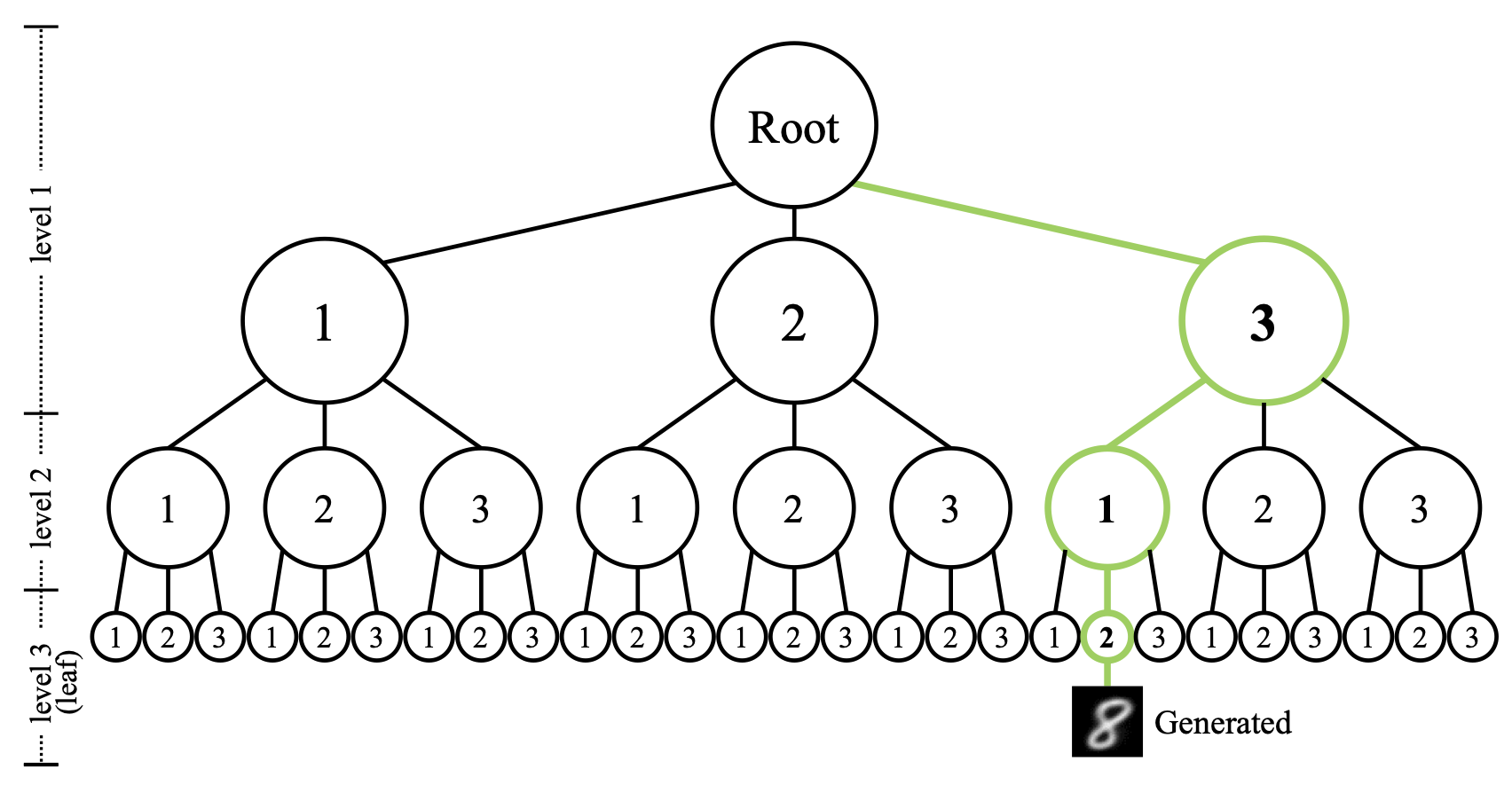
The training approach is also unique; to avoid some nodes from being under or over represented the authors propose a Split-and-Prune algorithm inspired by evolutionary selection: nodes matched too frequently get cloned; nodes rarely selected get pruned. The goal here is to have node selection chances uniformly distributed across the layer.

The discrete sampling also enables zero-shot conditional generation without gradient-based guidance. Since generation is just a sequence of discrete choices, one can guide the model's output with any discriminator by scoring each node's output, and then picking the best one.

The following is my exploration of the DDN paper, which also served as an opportunity to get familiar with the tinygrad library (my repo can be found under resources).

Normal Distribution Example

To build intuition, let's start simple: a 1D tensor of just 5 learnable parameters (nodes) trained to approximate a normal distribution. Each training step, we sample from the target, find the closest node to that target, and only that node gets updated via the error gradient.

But this then leads to a problem: some nodes get matched frequently, others rarely or never. These "dead nodes" would still get selected during generation, producing poor outputs. Meanwhile, high-density regions of the target distribution end up underrepresented.

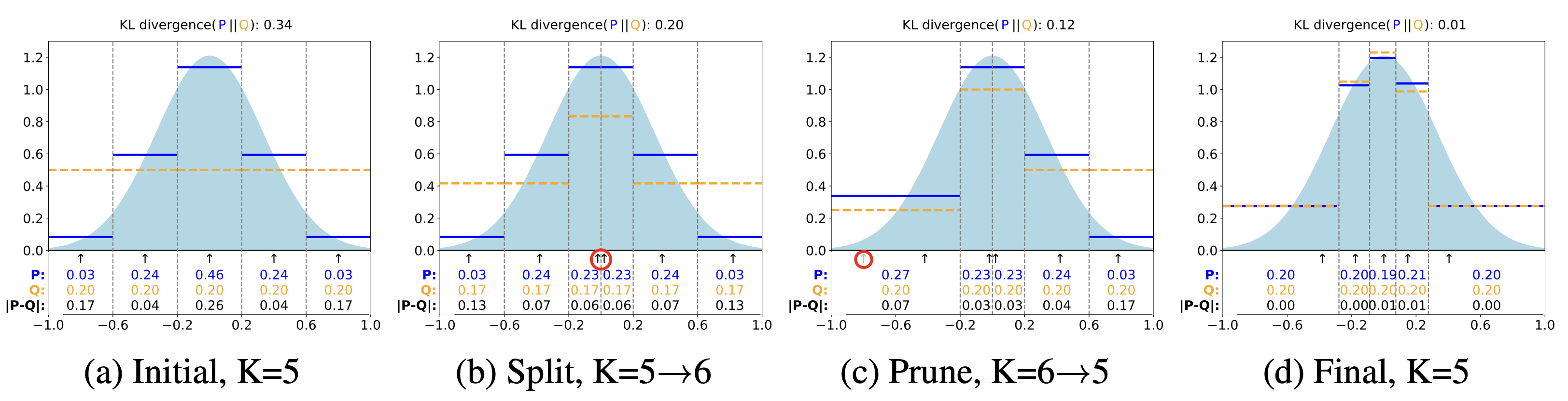Splitting and Pruning to move closer to the target distribution Figure from Yang, 2024

To remedy this we keep track of the selection counts of each node and if a node falls below a certain threshold ($0.5/K$ in the paper) it will get pruned. Similarly if a node exceeds a selection threshold ($2/K$), it will be split into two nodes with the same value. The figure above also illustrates how the KL divergence between the target P and the discrete approximation Q decreases as out of distribution nodes get split and pruned as their values update.

Implementation wise since we really can't (efficiently) dynamically increase or decrease the number of nodes we keep the number of nodes static; pruned nodes will cause the most selected nodes to split and replace them and splitting will cause the least selected nodes to be replaced/pruned.

Finally here's a training run with 10,000 nodes, to demonstrate how the discrete approximate the normal distribution fairly well as their number increases.

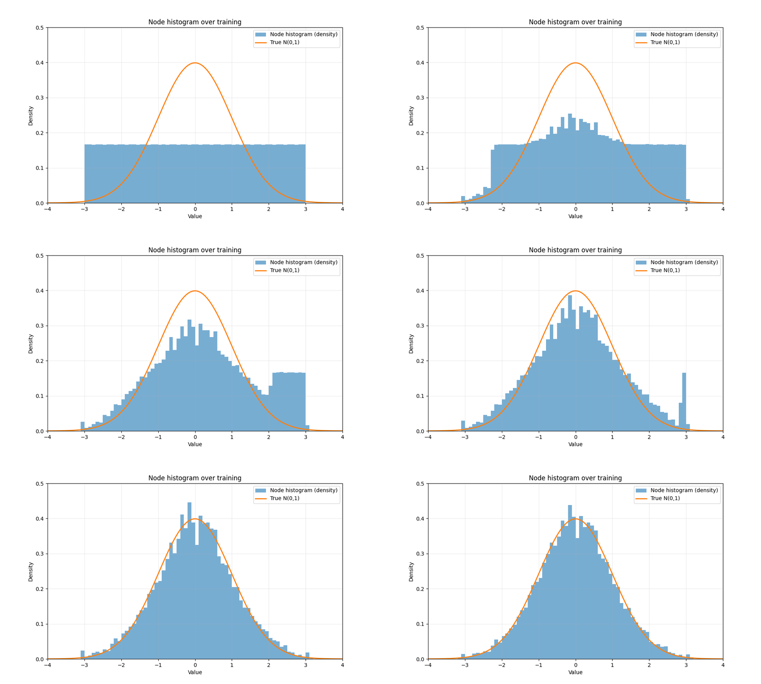
After training is complete the nodes cluster where probability density is high and uniform sampling over the trained nodes approximates the target distribution.

This same principle scales to images but instead of scalar parameters nodes become 1x1 convolutions that output image patches.

MNIST

Let's move on to a slightly more difficult dataset, MNIST. I opted to use a UNET architecture for the backbone, instead of the hierarchical architecture mentioned in the paper. I also ended up experimenting bit more with the architecture of the nodes, with my experiments laid out below.

Output Nodes (code)

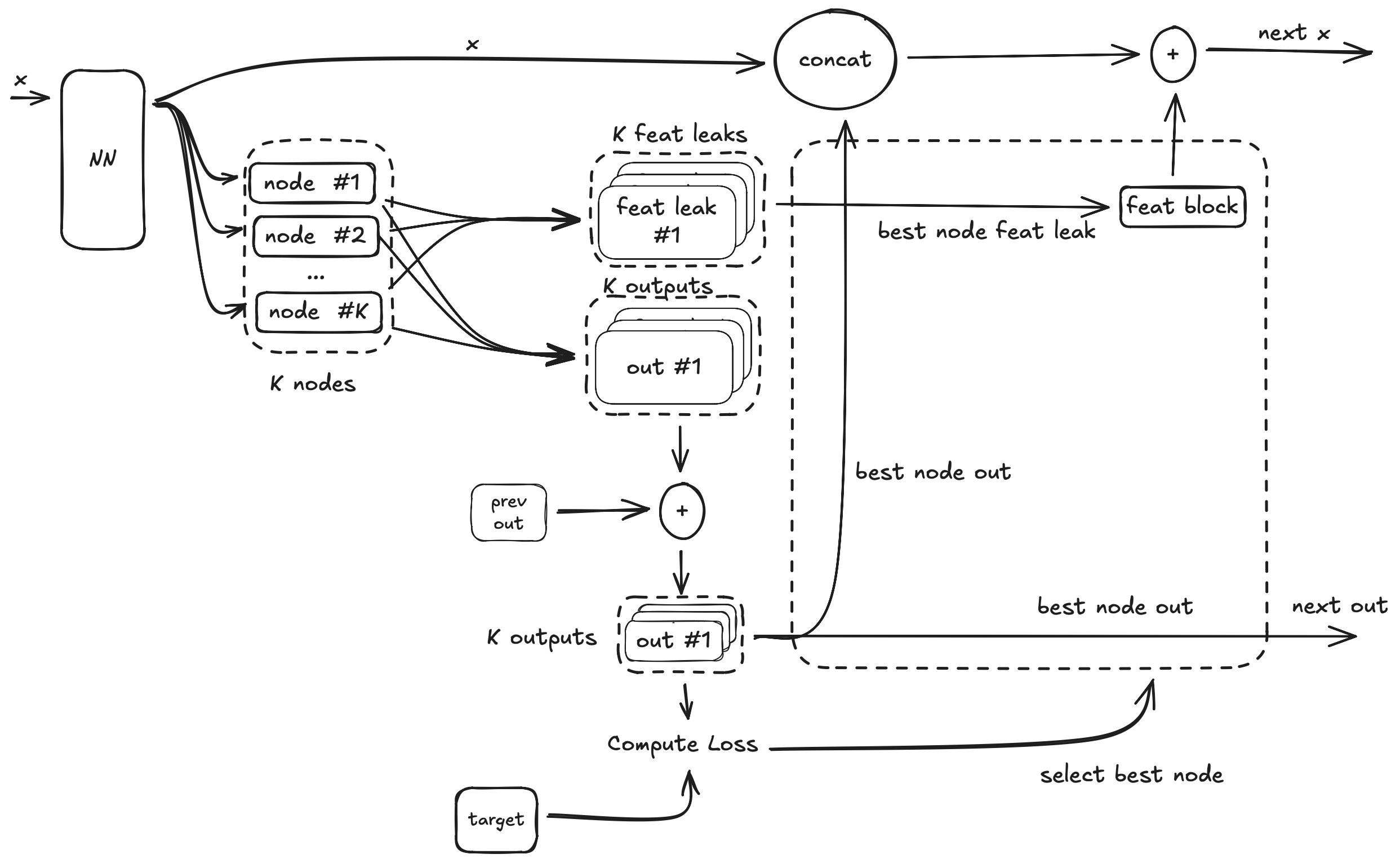
The paper's figures mainly show the basic output nodes, where each node acts as a decoder which maps from the feature space into the output space. The selected output, closest to the target gets then concatenated or added to the features to condition the next layers on the chosen node. By themselves output nodes don't work very well (as I also found in my experiments), that's why the author also proposes a "leak choice" where each node also produces some additional "features" which also get added to the features for conditioning. Additionally the authors add chain dropout, the nodes in each layer get chosen at random given a certain probability.

Feature Nodes (code)

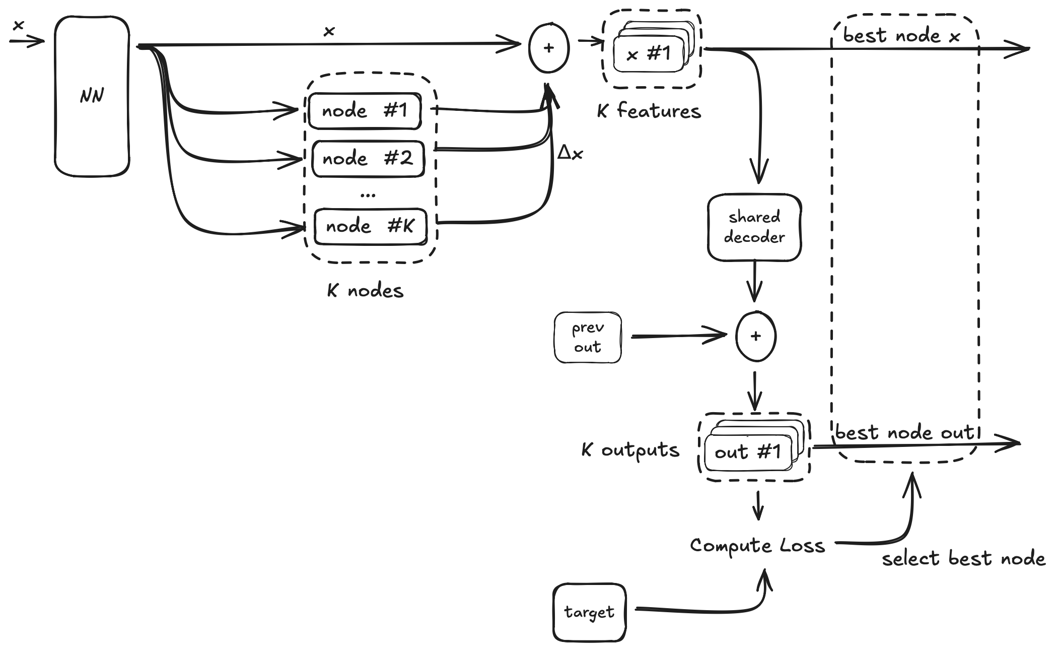
I figured with the original approach the nodes have to learn unique characteristic as well as mapping from feature/embedding space to output space. So instead I had the nodes directly map back to the embedding space, and a shared decoder translates the embeddings to output space. This obviously has the drawback that the nodes are larger since they go from feature to feature space instead of feature to output space, where the output dim is usually a lot smaller. The model does converge a lot quicker compared to the original architecture in terms of training steps. But it does seem overfit on the training data without adding chain drop out.

Latent/Bottlenecked Nodes (code)

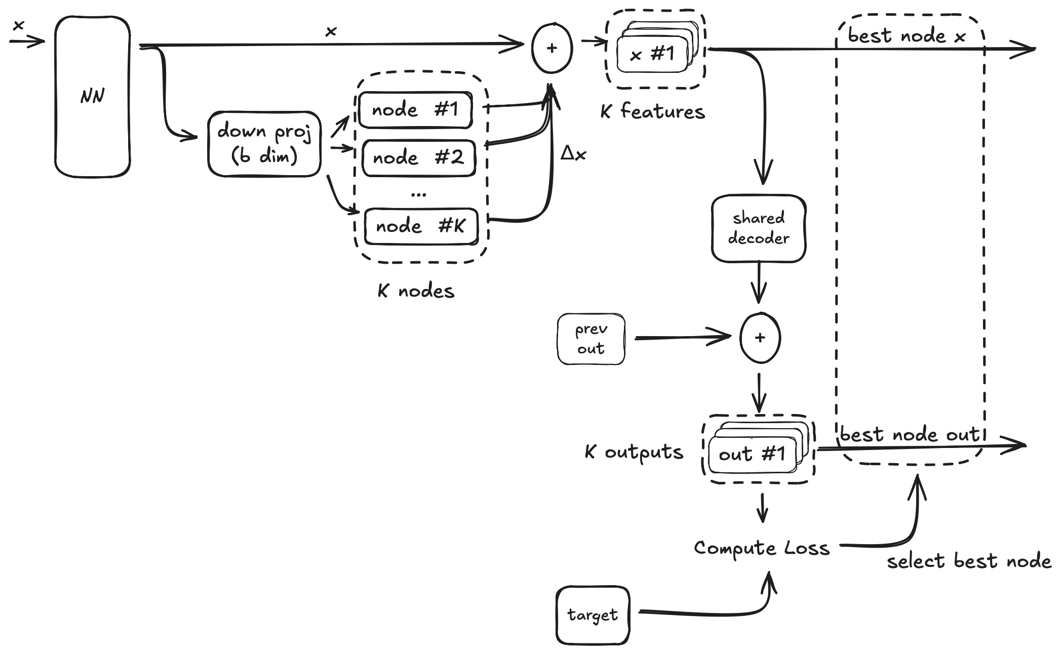
Attempting to tackle the above mentioned problem with the increase node size, we can instead compress the embedding dim through a bottleneck an then have the nodes act on this space before upcasting it back to the feature dim. This works as well as the full feature nodes, and doesn't seem to overfit even without chain dropout.

Comparison

All models share the same UNET backbone between the layers so they only differ in the actual DDN architecture. They all converge to a similar eval loss besides the feature nodes without chain drop, which most likely is overfitting on the training data. 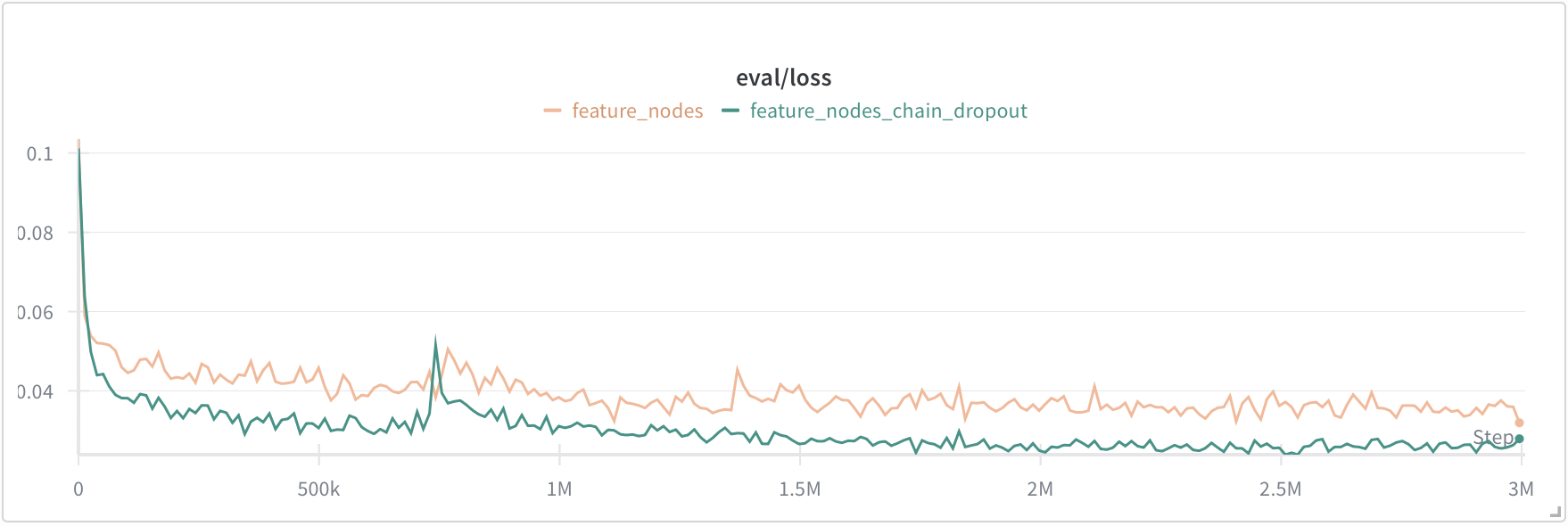feature nodes with and without chain dropout

Also the output nodes seem to converge a lot slower compared to the feature and bottleneck nodes. 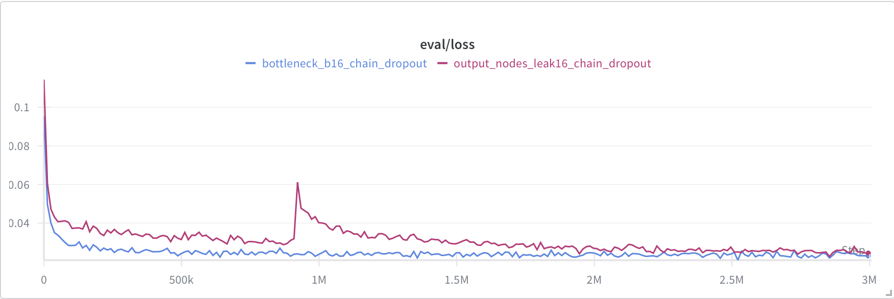comparison between bottleneck nodes and the output node with leak choice

Table with evaluation results and parameter counts:

Model	Test Loss	Parameters
bottleneck_b16	0.022420	5,683,878
bottleneck_b16 (with chain-dropout)	0.022293	5,683,878
feature_nodes	0.029651	8,036,934
feature_nodes (with chain-dropout)	0.022822	8,036,934
output_nodes_leak16	0.024325	6,418,464
output_nodes_leak16 (with chain-dropout)	0.022866	6,418,464

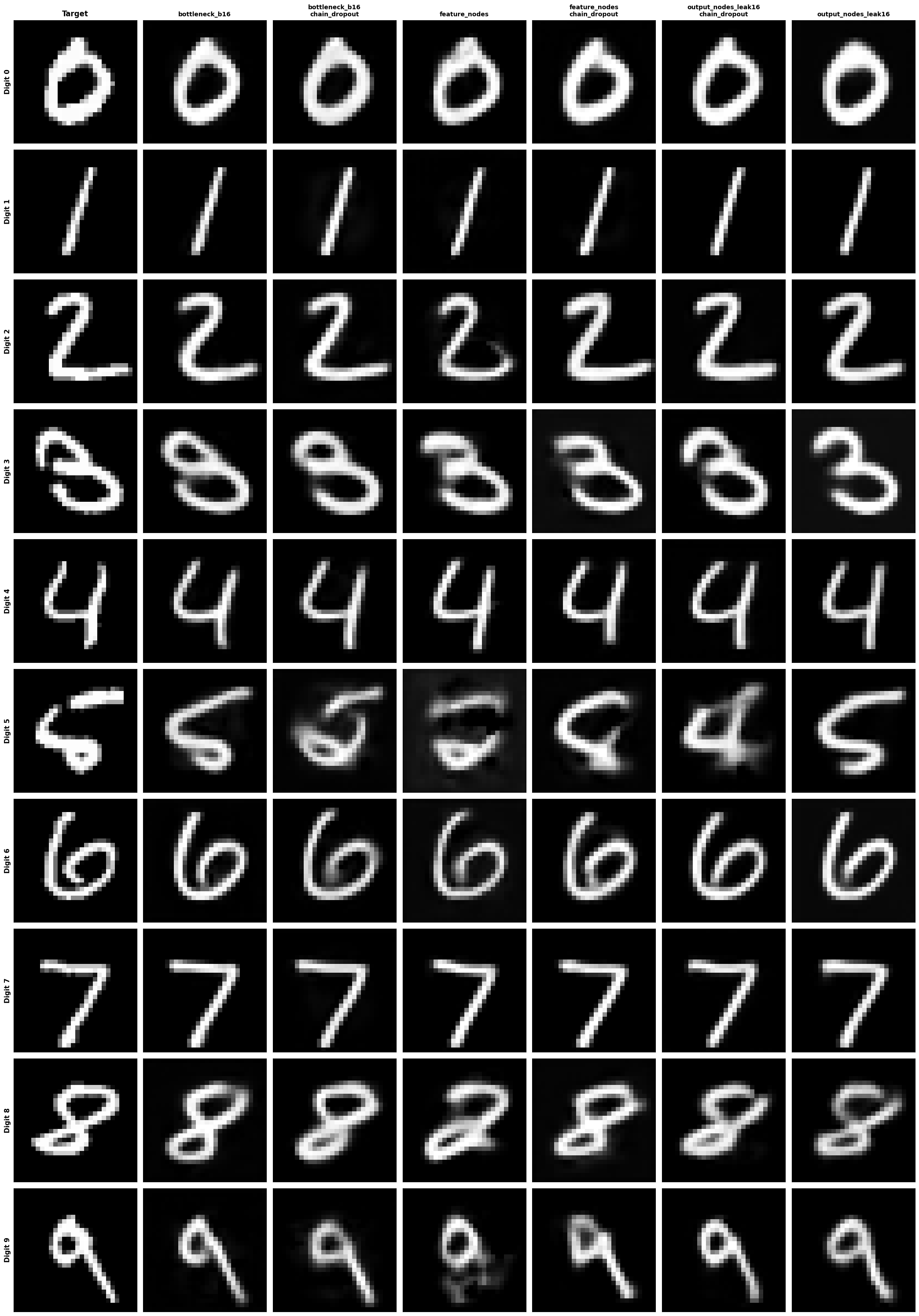Individual digits produced by each architecture

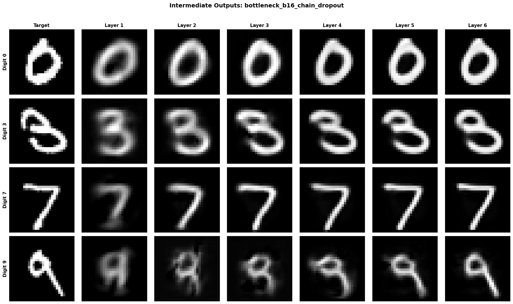Intermediate outputs of the bottleneck model at each layer

Zero-Shot Conditional Generation

The paper touts that the model can do guided generation without being explicitly trained to do so. This is done, by scoring the dd nodes output with an evaluator, this can be MSE loss with a target image, similar to training, or another network like clip. For a simple demonstration I just trained tinygrad's example mnist classifier and pass along with it a number we would like to generate. The classifier returns the class logits for each node 's output and we select the node whose current output is closest to our desired number.

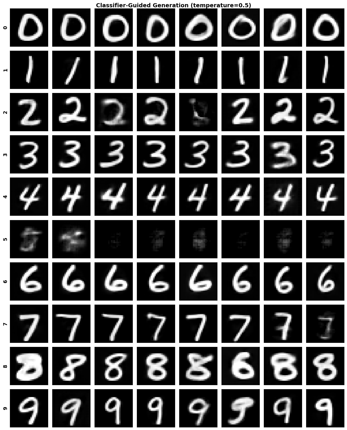temperature sampled numbers based on the classifier logits (bottleneck arch)

Beam Search

As you can see some numbers don't seem to come out quite right, which is probably due to the classifier struggling with the "half-baked" images of early layer outputs and makes us pick the wrong nodes that won't lead to satisfying outputs. Luckily since we are dealing with discrete sequential "decisions" we can utilize any tricks that have been developed for LLMs. Here I added beam search and our troubled numbers look a lot better now!

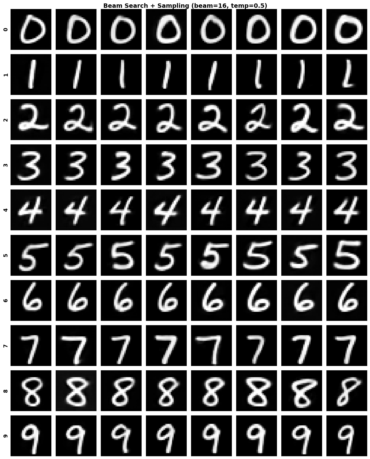(bottleneck arch) (You may notice that the outputs of the individual numbers now look a bit more samey than before, which is due beam search limiting the diversity of the outputs as it optimizes for the most probable.)

Finally what actually happens when we just do random sampling? Well... it does produce digits but the numbers are more hit or miss 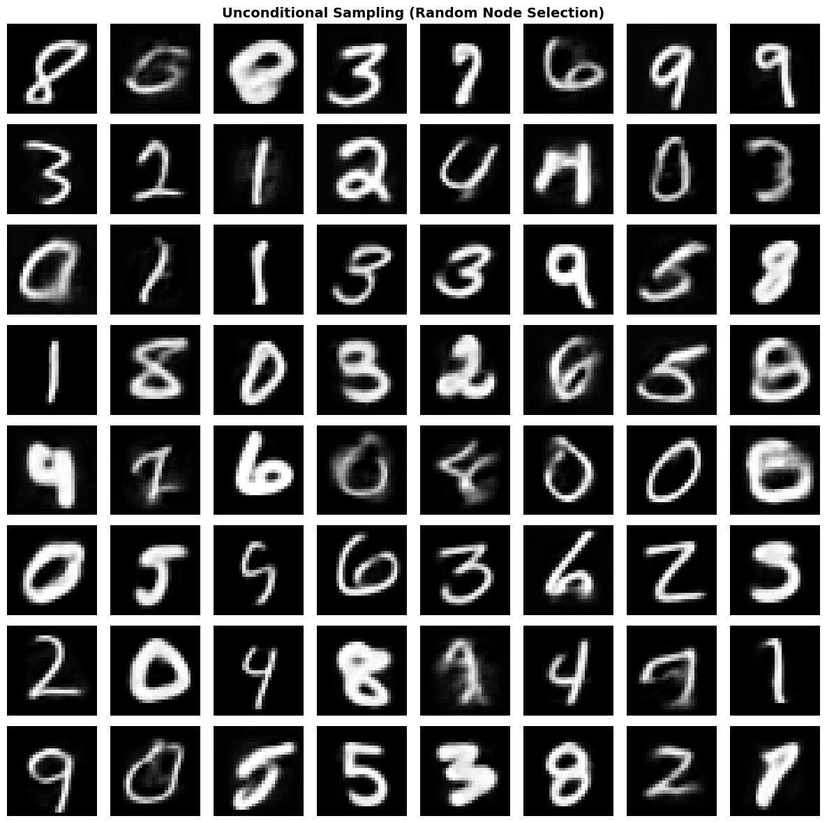(bottleneck arch)

What I learned

This concludes my exploration of the DDN paper, it definitely was a very novel idea which was fun to implement.

DDN

While I don't think the architecture will replace any of the current mainstream diffusion models, it's cool to see how such a unique architecture achieves reasonable outputs. The evolution-inspired approach to splitting and pruning was a highlight. One of the reasons why I don't think this approach will find mainstream appeal is that guided generation requires evaluating all K nodes at each layer, which gets expensive.

Some optimizations I'd recommend for future work within Tinygrad: two-pass bottleneck selector: in Pass A (no-grad) score nodes in output space in small chunks, updating an argmin, so you never materialize the full feature tensor for all nodes since we only need it from one node for the next layer. In Pass B (with grad) recompute only the selected node(s) in feature space (e.g., via grouped 1×1 conv) and run the real decoder/backprop.

I also noticed loss spikes occurring around the same training steps across all runs — could be worth investigating.

TinyGrad

A few lessons from implementing this in tinygrad:

- In-place operations break silently in jitted code: things like `/=` would fail without error, which was tricky to debug. Tbh this more of a noob mistake on my end. - Advanced indexing doesn't play well with multi-GPU: After I had split and prune working well, I started training on multiple GPUs which completely broke the process again and I had to reimplement without advanced indexing. - The node kernel is the compute bottleneck: especially for feature and bottleneck variants, it uses a lot of memory. The output nodes can be more easily optimized as one only has to evaluate the output, and then select the leak features of the node. - Making split-and-prune jittable was tricky: but not the main performance bottleneck once done.

Resources

- Paper - Personal Project Github - Official Github - lucidrains github - 10K node demo