The common residual stream has become a cornerstone of deep learning. Each layer's output is added back into a running sum, gradients flow, deep models train without collapsing. But that same additive trick has a hidden consequence: the residual's norm grows with depth, and as it grows, later layers have to push harder just to move it. The result is that many of your deep layers end up barely changing anything. _Scaling Adaptive Depth with Norm-Agnostic Residual Networks_ proposes a geometrically elegant solution, separating the residual's direction from its magnitude and managing the two independently. This gives every layer explicit control over how much it changes the residual, while also producing some interesting side effects, such as a built-in confidence signal, less reliance on attention sinks, and a natural route toward adaptive-depth computation. The paper looks fairly dense at first, but the central geometry is surprisingly simple. Assuming you're comfortable with the basics of how a transformer works, I’ll build up that intuition step by step, then look at the paper’s results and what I learned when I implemented NAG myself.

The Residual Stream

First off, it's worth understanding why residual streams have become ubiquitous in modern neural networks, what problems they solve and if their current implementations are optimal.

Residual streams are pretty much a given in modern neural networks because they make deep models much easier to train. They give information an identity path through the network and, during backpropagation, give gradients a direct route that does not depend entirely on multiplying through every layer. This allows each layer to focus on adding a useful update, rotating the residual and/or changing its norm, without also having to relearn how to preserve everything it should leave unchanged.

To demonstrate, let’s see what happens when we stack random layers with and without a residual connection and track the activation norm. Each layer multiplies by a random matrix $W_l$ with small (sub-unit) singular values; the non-residual network computes $x_{l+1} = W_l x_l$, the residual one $x_{l+1} = x_l + W_l x_l$.

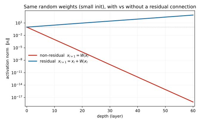
In this toy setup, the signal without a residual connection decays exponentially; after 60 layers its norm has collapsed by ~18 orders of magnitude. The signal is effectively gone. Gradients pass through the same shrinking product, so they vanish for exactly the same reason. With the residual connection, the identity path means that neither the forward signal nor the gradient depends entirely on that long matrix product.

The Problem

Yet this solution creates a problem of its own: the residual norm tends to grow unchecked with depth. As that norm grows, deeper layers must produce larger outputs to rotate or otherwise modify the residual by the same relative amount. The relative contribution of deeper layers often becomes smaller as a result. This could reflect useful behavior, with later layers making increasingly fine-grained refinements; other work, such as the recent Tapered LLMs paper, offers a different interpretation of this phenomenon. The Norm-Agnostic Residual Networks paper, however, argues that at least part of it is an architectural bias rather than an intentional feature. Since deeper layers cost roughly the same number of FLOPs as earlier ones, systematically suppressing their influence would represent wasted capacity.

Transformers mainly differ in where they normalize the residual stream relative to each sublayer:

Post-Norm

In post-norm, the layer receives the unnormalized residual, outputs its update, and the combined residual-plus-update is normalized before being passed to the next layer:

$ R_{l+1} = \text{Norm}(R_l + f_l(R_l)) $

This keeps the residual scale controlled, but it prevents the raw overall magnitude from being carried forward as an independent signal. Learnable scale and shift parameters can reintroduce some magnitude information, although less directly. Post-norm is still used in recurrent reasoning methods like TRM and EqR, where repeatedly reusing the same block makes controlling the scale of the recurrent state especially important.

Pre-Norm

Pre-norm is the most common arrangement in modern Transformers. The residual is normalized before being passed to the layer:

$ R_{l+1} = R_l + f_l(\text{Norm}(R_l)) $

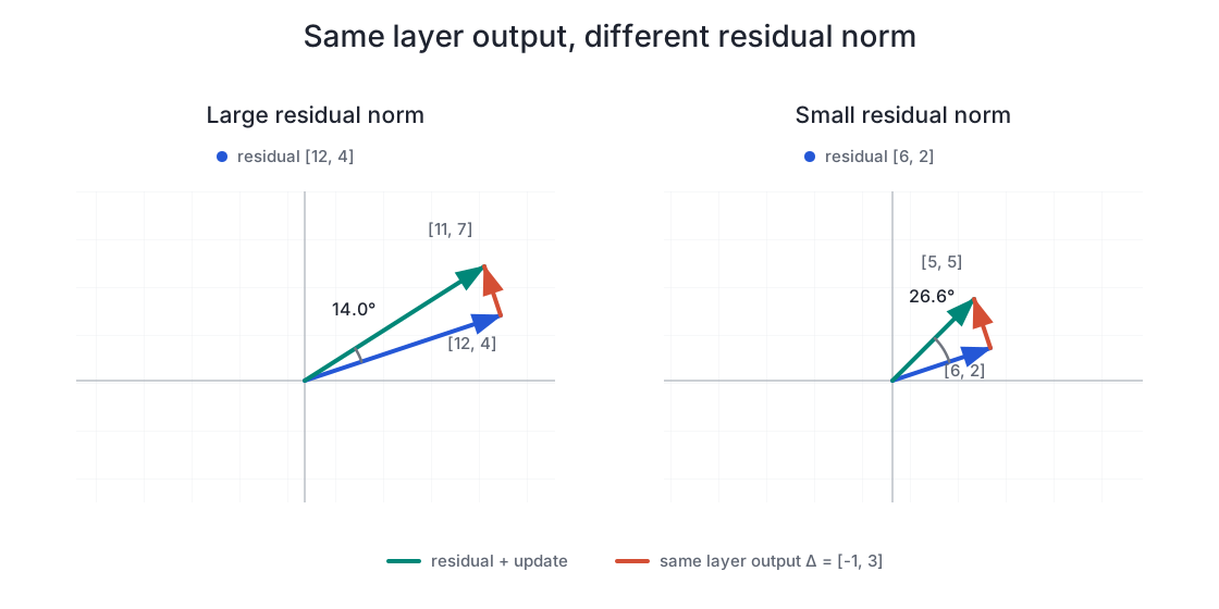
While this makes the layer invariant to the input’s norm, it also hides potentially useful information from the layer: two residuals that point in the same direction but have very different magnitudes look identical after normalization, so the layer produces the same update for both. Once added back into the residual stream, however, that update can have a much larger relative effect on the smaller residual than on the larger one. The layer has no direct access to the residual magnitude it would need to calibrate this update.

For a simple numerical example, suppose both residuals are rescaled to the same reference vector before entering the layer. The particular scale is chosen for clean arithmetic:

Layer’s effect on a large-norm residual

$ \begin{aligned} Res = [12, 4] \\ \to \operatorname{Rescale}(Res) = [3, 1] = LayerInput \\ \to Layer([3, 1]) = [1, 2] = LayerOutput \\ \to Res = Res + LayerOutput = [13, 6]\\ \end{aligned} $

Layer’s effect on a small-norm residual

$ \begin{aligned} Res = [6, 2] \\ \to \operatorname{Rescale}(Res) = [3, 1] = LayerInput \\ \to Layer([3, 1]) = [1, 2] = LayerOutput \\ \to Res = Res + LayerOutput = [7, 4]\\ \end{aligned} $

The Solution: Norm-Agnostic (NAG) Residual Stream

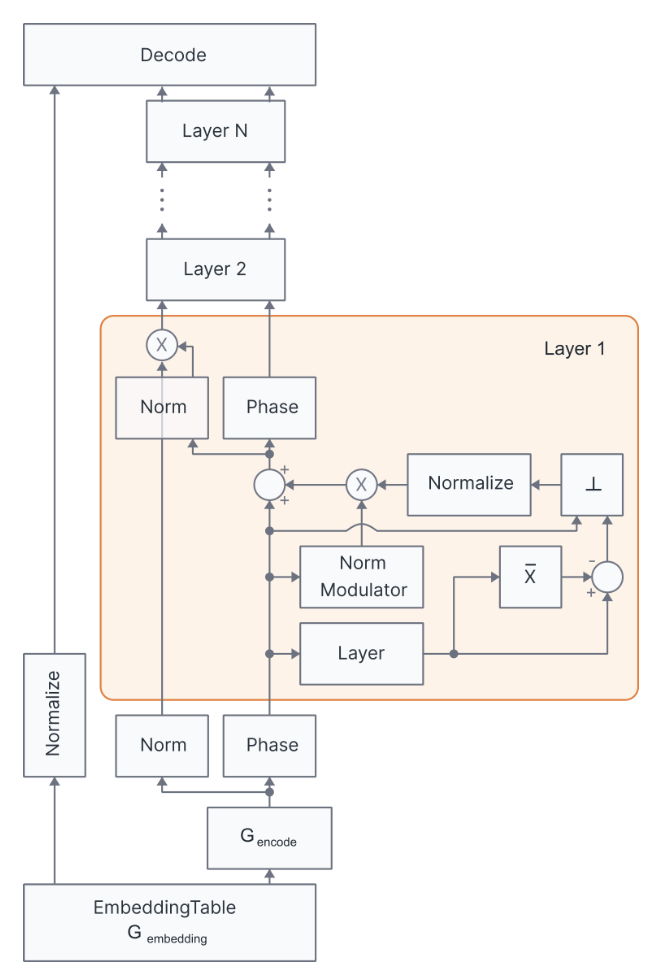
The paper’s solution is to disentangle the residual’s direction from its magnitude, creating two streams: a normalized direction $\bar{R}_l$ and a scalar magnitude $\rho_l$.

$ R_l = \rho_l \bar{R}_l $

The direction stream is kept at RMS one, placing $\bar R_l$ on a hypersphere of radius $\sqrt d$. Each token embedding is split into its initial direction and magnitude; subsequent layers keep the direction on the hypersphere while tracking the accumulated magnitude separately.

NAG first centers each layer’s output by subtracting its feature-wise mean, then removes the component parallel to $\bar R_l$ (from here on, $f_l(\bar R_l)$ denotes this centered layer output). Since a parallel component changes the residual’s magnitude without adding new directional information, removing it leaves only the component that can rotate the residual.

To remove this redundant part, we first measure how much the layer output points in the same direction as the residual. The dot product $\left\langle f_l(\bar{R}_l), \bar{R}_l \right\rangle$ measures their overlap, and dividing by the residual’s squared length $\left\lVert \bar{R}_l \right\rVert_2^2$ turns that overlap into a multiplier:

$ \frac{ \left\langle f_l(\bar{R}_l), \bar{R}_l \right\rangle }{ \left\lVert \bar{R}_l \right\rVert_2^2 } $

Multiplying that number by the residual direction gives us the layer output’s “shadow” along the residual—formally, its parallel projection.

$ \text{vector parallel to the input residual} = \frac{ \left\langle f_l(\bar{R}_l), \bar{R}_l \right\rangle }{ \left\lVert \bar{R}_l \right\rVert_2^2 } \bar{R}_l $

We can then subtract this shadow from the layer output, which leaves only the part pointing at a right angle to the residual: the orthogonal component.

$ f_l^{\perp}(\bar{R}_l) = f_l(\bar{R}_l) - \frac{ \left\langle f_l(\bar{R}_l), \bar{R}_l \right\rangle }{ \left\lVert \bar{R}_l \right\rVert_2^2 } \bar{R}_l $

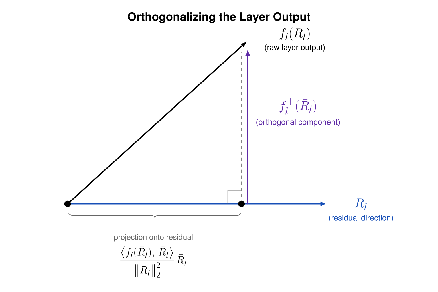This changes the role of the layer: it can now only directly _turn_ the residual, rather than scale it along its current direction. The residual update equation becomes:

$ R_{l+1}= \rho_l(\bar{R}_l + f_l^{\perp}(\bar{R}_l)) $

Early in training, however, layer outputs are often highly aligned with the residual direction. Removing that parallel component can leave a very small orthogonal update, weakening the layer’s contribution and hurting sample efficiency. To give this remaining update a consistent scale, NAG normalizes it to have an L2 norm of $\sqrt d$:

$

N_{\mathrm{out}}(x) = \sqrt{d} \frac{x}{||x||_2} $

Normalizing every orthogonal update to the same length solves the small-update problem, but it also makes every layer contribute at the same scale for every token. Motivated by prior work on latent MoEs and Zyphra’s CCA showing that computation can remain effective in low-rank spaces, the authors hypothesize that each layer specializes in a set of preferred directions. When the residual aligns with those directions, the layer should contribute more; when it does not, its update should be suppressed.

NAG therefore introduces two controls: a modulator $m_l(\bar R_l)\in[0,1]$, which decides how much the layer should contribute for the current token, and a learned scalar $\alpha_l$, which sets that layer’s maximum contribution.

To let the modulator learn a set of preferred directions, we give each layer $C$ learned direction vectors $w_{li}$, where $C$ is a hyperparameter. Each vector acts like a compass direction in the normalized residual space. For each one, the projection

$ \bar R_l^\top w_{li}+b_{li} $

measures how well the current residual direction aligns with that preference, with the bias controlling where the preference begins to activate. A sigmoid $\sigma$ turns this into a soft gate between zero and one. Geometrically, each gate therefore defines a soft region of the hypersphere where the layer should contribute more strongly.

The learned softmax weights $p_{li}$ combine these regions into the layer’s overall preference, while ensuring the result remains between zero and one. Finally, the positive exponent $\beta_l$ controls how selective that preference is: values above one suppress partial matches, while values below one make them count more strongly.

Thus the full parametrization of $m_l$ is:

$ m_l(\bar{R}_l) = \left( \sum_{i=0}^{C-1} p_{li}\sigma\left(\bar{R}_l^\top w_{li} + b_{li}\right) \right)^{\beta_l} $

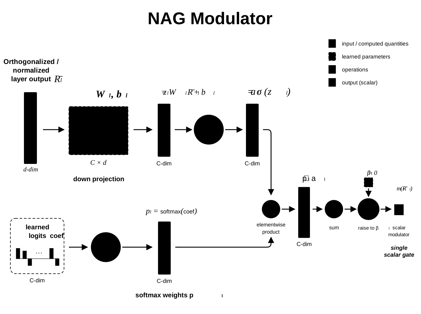
This resembles an MoE router: both learn directions in residual space that determine when a computation should be emphasized. When applying the modulator to MoE layers, the authors set $C$ to at least the number of experts, giving it enough directional capacity to represent expert-specific preferences.

At this point, we have all the main pieces. Putting them together gives the full update:

$ R_{l+1}= \rho_l\bar{R}_l + \rho_l \alpha_l m_l(\bar{R}_l) N_{\mathrm{out}}(f_l^{\perp}(\bar{R}_l)) $

Since $\bar{R}_l$ and $N_{\mathrm{out}}(f_l^{\perp}(\bar{R}_l))$ are orthogonal, the update forms a right triangle, with $\|\bar{R}_l \|$ being the adjacent leg, $\| \alpha_l m_l N_{\mathrm{out}}(f_l^{\perp}(\bar{R}_l)) \|$ the opposite leg, and the updated (unnormalized) residual being the hypotenuse:

$ \begin{aligned} R_{l+1}= \rho_l(\underbrace{\bar{R}_l + \alpha_l m_l(\bar{R}_l) N_{\mathrm{out}}(f_l^{\perp}(\bar{R}_l))}_{\text{hypotenuse}}) \\ \end{aligned} $

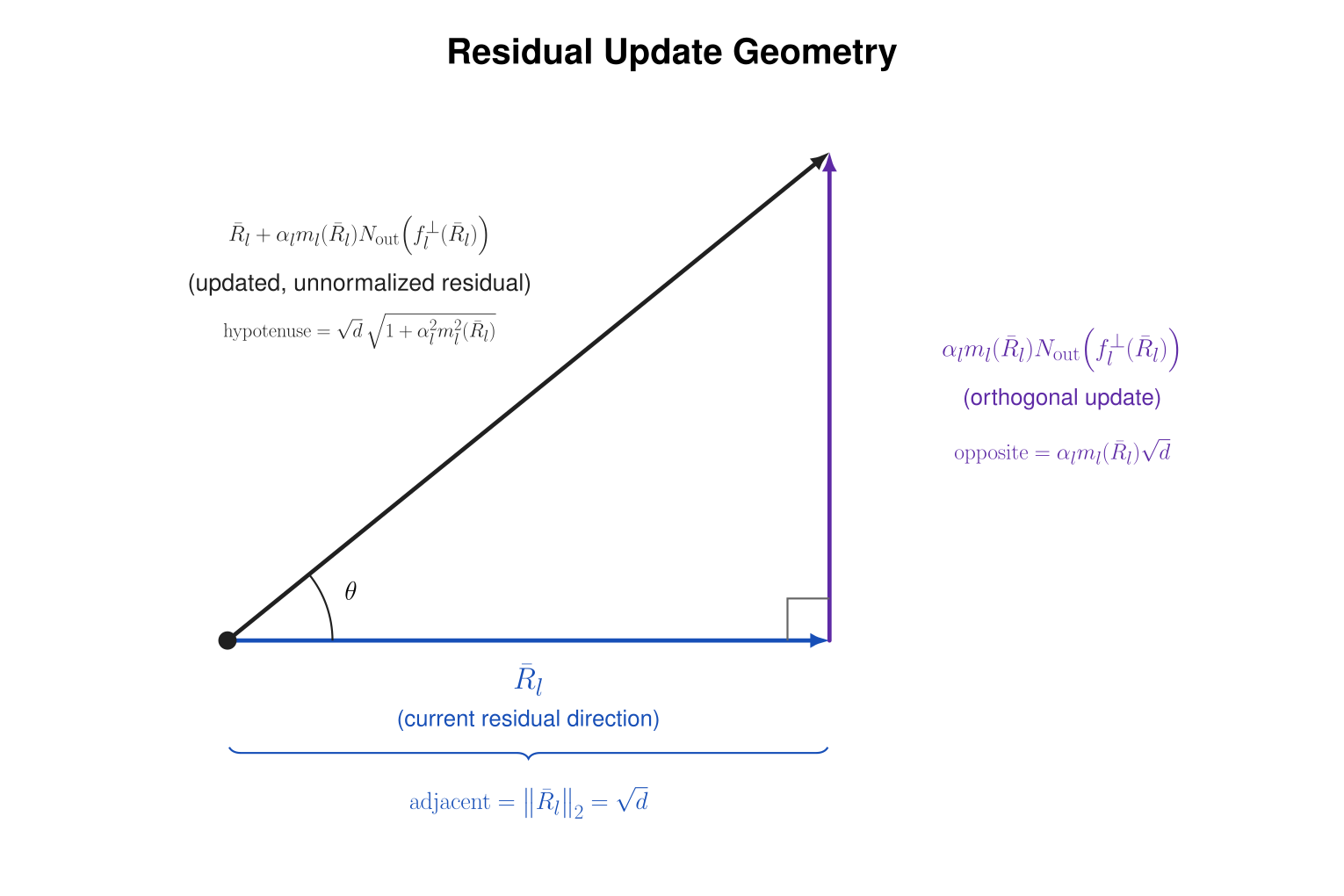That triangle gives us the rotation angle immediately: the ratio of the opposite leg to the adjacent leg is $\tan\theta$:

$ \tan \theta = \frac{\mathrm{opposite}}{\mathrm{adjacent}} = \frac{\left\lVert \alpha_l m_l(\bar{R}_l) N_{\mathrm{out}}(f_l^{\perp}(\bar{R}_l)) \right\rVert}{\left\lVert \bar{R}_l \right\rVert} = \frac{\alpha_l m_l(\bar{R}_l) \sqrt{d}}{\sqrt{d}} = \alpha_l m_l(\bar{R}_l) $

The product $\alpha_lm_l(\bar R_l)$ tells us how large the orthogonal update is relative to the current residual direction. This makes the roles introduced earlier concrete: $m_l$ chooses how much of the layer’s available update to use for this token, while $\alpha_l$ sets the ceiling.

The same triangle now does double duty: its angle gives us the rotation, while its hypotenuse gives us the norm growth. Because the vector sum forming the hypotenuse is the updated direction before renormalization, its length follows directly from the Pythagorean theorem:

$

\|\bar{R}_l + \alpha_l m_l(\bar{R}_l) N_{\mathrm{out}}(f_l^{\perp}(\bar{R}_l))\| = \sqrt{d + \alpha^2_l m^2_l(\bar{R}_l) d} = \sqrt{d}\sqrt{1 + \alpha^2_l m^2_l(\bar{R}_l)} $

Computing the norm of the updated residual gives us:

$

\| R_{l+1} \| = \rho_l\sqrt{d}\sqrt{1 + \alpha^2_l m^2_l(\bar{R}_l)} $

$ \rho_{l+1}\sqrt{d}= \rho_l\sqrt{d}\sqrt{1 + \alpha_l^2 m_l^2(\bar{R}_l)} $

Now we can drop $\sqrt{d}$ from both sides and divide by $\rho_{l}$ to get the rate of change of the norm:

$ \text{norm gain} = \frac{\rho_{l+1}}{\rho_{l}}= \sqrt{1 + \alpha_l^2 m_l^2(\bar{R}_l)} $

The same $[0,1]$ bound on $m_l$ means $\alpha_l$ also caps the per-layer norm gain (maxing at $\sqrt{1 + \alpha_l^2}$). So a single learnable scalar per layer, $\alpha_l$, sets the ceiling on how much that layer can both rotate and grow the residual, while $m_l$ decides how much of that ceiling to spend on each token.

Knowing the norm gain per layer, the full norm-agnostic residual stream update becomes two equations:

1. The direction-residual update, now divided by the norm gain to keep the vector normalized:

$ \bar{R}_{l+1}= \frac{\bar{R}_l + \alpha_l m_l(\bar{R}_l) N_{\mathrm{out}}(f_l^{\perp}(\bar{R}_l))}{\sqrt{1 + \alpha_l^2 m_l^2(\bar{R}_l)}} $

2. The norm residual update

$ \rho_{l+1} = \rho_l \cdot \sqrt{1 + \alpha_l^2 m_l^2(\bar{R}_l)} $

For numerical stability the norm residual scalar $\rho_l$ is stored in log space $s_l = \log \rho_l$. And so the update equation becomes:

$ s_{l+1} = s_l + \frac{1}{2} \log(1 + \alpha_l^2 m_l^2(\bar{R}_l)) $

These two equations are applied after every attention and MLP update. The direction residual and norm scalar then travel through the Transformer until we reach the final direction $\bar{R}_L$ and norm $\rho_L = e^{s_L}$, where $L$ denotes the final layer. At decoding $\bar{R}_L$ is multiplied against the normalized output embedding table, producing cosine similarities per token. Because the token cosine similarities sit in the $[-1, 1]$ range the raw softmax over them would be very flat. What we need is to scale up the values to sharpen the distribution. Now that's where the final norm scalar $\rho_L$ takes effect; before computing the softmax onto the cosine values to get the final token generation probabilities $P$, the residual norm is applied as an inverse temperature.

$ T_{eff} = \frac{1}{\rho_L} = \frac{1}{e^{s_L}} $

$ P = \mathrm{softmax}(\frac{\text{cos-sims}}{T_{eff}}) = \mathrm{softmax}(\rho_L \cdot \text{cos-sims}) $

The norm therefore acts as a learned, token-dependent inverse temperature, which can be interpreted as a confidence signal. For a fixed set of cosine similarities, a larger norm produces a sharper output distribution, while a smaller norm leaves it flatter. This gives us a single “confidence” scalar per token that we can track as it evolves through depth!

Note that the original embedding table, while centered, is not strictly normalized and so carries its own norm $G_{embedding}$. Additionally the authors also apply a gain $G_{encode}$ to the embedding norm before splitting the residual into direction and norm, so the temperature is composed of

$ T_{eff} = \frac{1}{G_{embedding}\cdot G_{encode}\cdot G_{travel}} $

Paper Results

So, does any of this actually help? The authors train a family of ~150M-active / 900M-total-parameter MoE Transformers on 50B tokens. They vary the width-to-depth ratio while keeping the parameter count fixed; a smaller ratio means a deeper model. A standard residual MoE is trained alongside each NAG model.

The figure below shows a NAG loss advantage that grows with depth, from roughly 0.012 nats at ratio 80 to roughly 0.028 at the deepest ratio of 20. 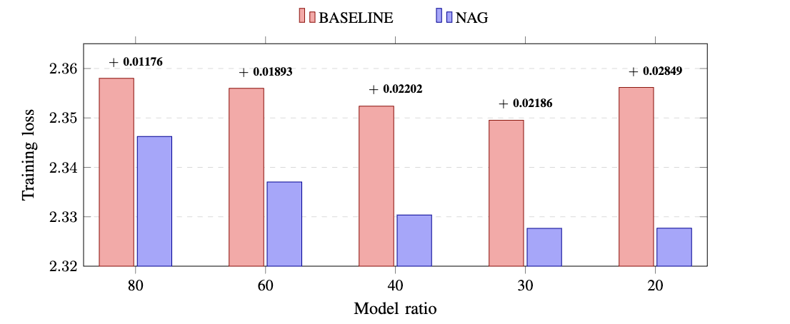Another feature of NAG is that it allows the attention layers to handle attention sinks differently. To quickly recap, an attention sink is a token, usually the first token, BOS, that many later tokens attend to even when it carries little contextually useful information. It can act like a learned “null” destination: since softmax has to put its probability mass somewhere, a head with little useful information to add can dump it there, as long as the resulting value write has little effect. The paper hypothesizes that NAG reduces the need for this workaround. Because the modulator can suppress the entire attention branch when it has little to contribute, the model has less pressure to route unused attention mass into the BOS token. 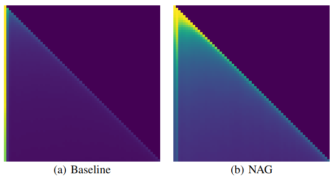The gains are small, only hundredths of a nat, but they remain consistent as depth increases. The NAG architecture has another consequence which an attentive reader may have already caught. Going back to how the Residual direction and norm get updated. When $m_l \approx\ 0$ , predicting that the layer will do basically nothing, the effective update becomes:

$ \begin{aligned} R_{l+1} = R_l \\ s_{l+1} = s_l \end{aligned} $

So why expend the valuable compute at all?

Mixture-of-Depths (MoD)

NAG's architecture has a natural path to adaptive depth compute. Since $\alpha_l m_l$ estimates how much the layer will rotate the residual, it can be used as a natural skip score. We mainly have to find a generalizable way to apply it across layers. If the predicted rotation is tiny, executing the full layer is unlikely to change the representation much. Recalling the directional residual update computation we did earlier $\tan \theta_l =\alpha_l m_l(\bar{R}_l)$, we can retrieve the exact angle that the residual will be rotated by a layer with:

$ \theta_l = \arctan(\alpha_l m_l(\bar{R}_l)) $

And since the learned $\alpha_l$ dictates the maximum rotation, the maximum rotation is just:

$ \theta_l^{max} = \arctan(\alpha_l) $

This means we can divide the layer's rotation by its maximum possible rotation to create a normalized rotation score $r_l$:

$ r_l = \frac{\arctan(\alpha_l m_l(\bar{R}_l))}{\arctan(\alpha_l)} \in [0, 1] $

This normalized rotation score allows us to set an "activation" threshold in a well-defined range. We can then set a skipping threshold $p_{thres}$ that determines, from the modulator output, whether we compute the layer or not:

$ \begin{aligned} r_l &> p_{\mathrm{thres}} \to \text{execute layer } l \\ r_l &\le p_{\mathrm{thres}} \to \text{skip layer } l \end{aligned} $

Due to the skipping being tied to the modulator, the skip threshold has a geometrically meaningful interpretation: when does a rotation become worth paying for with compute? Unlike standard MoD, which trains a separate router network to decide when a layer gets skipped, here the skip score comes straight from the rotation geometry without requiring a dedicated router. One subtle issue arises: the skip creates a sharp transition. A layer whose rotation score is barely above the threshold gets a full layer update, while a score a little below doesn't cause an update. This can create sharp residual transitions between layers. To smooth the transition, the paper adds a learned vector $\vec{X}_l$ that is always applied even when the layer gets "skipped", basically acting as a base direction.

$ \hat{f}_l(\bar{R}_l) = \begin{cases} f_l(\bar{R}_l) + \vec{X}_l, & r_l > p_{\mathrm{thres}} \\ \vec{X}_l, & r_l \le p_{\mathrm{thres}} \end{cases} $

Even when a token skips the attention computation, its key and value vectors are still produced and cached so that future tokens can attend to it. Attention skipping therefore reduces computation but does not reduce the KV-cache size. Because the skipping mechanism is coupled to the modulator's geometry, it can be applied not just at inference time to save compute, but during pre-training as well. Under a fixed FLOP budget, compute saved by skipping low-impact layers can be reinvested into training on more tokens, while keeping the parameter count fixed. In a sense, NAG introduces depth sparsity as a new scaling axis, the same way MoE did for width. Under equal training FLOPs, the 20% MoD run processed 60.9B tokens instead of 50B and finished only 0.00055 loss behind the full-depth NAG model.

My Experiments

I implemented NAG in Karpathy’s nanochat and trained a 64-block, roughly 359M-parameter GPT model. Compared with the paper, I used a dense Transformer instead of an MoE, untied output embeddings, standard attention instead of CCA, and trained for roughly 10B tokens rather than 50B. I left out the MoD modifications. For a cleaner comparison, I also removed nanochat specific architectural tweaks from the baseline, including the smear gate and residual skip connections. I used the repository’s FLOP-scaling utilities to match total training FLOPs between my NAG and baseline runs. I hit some initial failures when trying to train NAG-GPT:

Failure 1: To Infinity

My first attempt encountered NaNs during training. I traced them to the modulator’s sigmoid underflowing to zero in bf16, which made the weighted sum inside the modulator equal to zero. If we call that weighted sum $u$:

$ m_l(\bar R_l) = \left( \underbrace{ \sum_{i=0}^{C-1} p_{li}\sigma\left(\bar R_l^\top w_{li}+b_{li}\right) }_{u} \right)^{\beta_l} $

During backpropagation, the derivative with respect to $u$ is:

$ m=u^\beta \qquad\Longrightarrow\qquad \frac{\partial m}{\partial u} = \beta u^{\beta-1} $

When $u=0$ and $\beta<1$, the derivative raises zero to a negative power, producing an infinite or undefined gradient. Clamping $u$ to a minimum of $10^{-6}$ before applying the exponent fixed it.

Failure 2: Shut Gates

On the second training run, almost a quarter of the residual updates were effectively shut off when their applied scale $\alpha_l m_l$ collapsed toward zero. Short ~75min ablations isolated early injection noise as the cause. Because nanochat’s output projections are initialized at zero, their first nonzero outputs are tiny and poorly learned. $N_{\mathrm{out}}$ immediately expands those outputs to a norm of $\sqrt d$, turning weak, noisy directions into full-sized noisy residual updates. In turn, the modulators responded by suppressing those updates; once their applied scale approached zero, the corresponding sublayers received too little gradient to recover. Lowering the modulator’s learning rate and gradually warming up $\alpha_l$ prevented the gates from slamming shut. I diagnosed and fixed these issues using two RTX 5090s before launching the final runs on eight H100s. Before committing to the final H100 run (and potentially wasting the compute on another failure), I tested the changes on two FLOP-matched pairs at smaller scale: depth 26 with $10^{18}$ and $3\times10^{18}$ FLOPs. As the budget tripled, the NAG–GPT validation gap shrank from 0.038 to 0.016. A rough extrapolation from this catch-up behavior and the much flatter end-of-run slope at depth 64 predicted a final gap of 0.002–0.010, corresponding to a NAG validation bpb of 0.752–0.760 against GPT’s known 0.7503. A short depth-64 pilot supported that range, as did the final run shown below.

Results

With the training issues solved, NAG-GPT finally behaved! The baseline GPT still achieved lower training loss and validation bpb, but NAG performed better on CORE: 0.237 versus 0.222. The training loss gap appears largely driven by NAG converging more slowly early in training, though it narrowed later. Given that trend and the paper’s longer 50B-token training runs, it is possible that NAG would also catch the baseline in validation bpb with more training, though this experiment does not establish that.

Run	Validation bpb ↓	CORE ↑
GPT baseline	0.7503	0.2225
NAG	0.7589	0.2373
NAG, broken	0.7858	0.2010

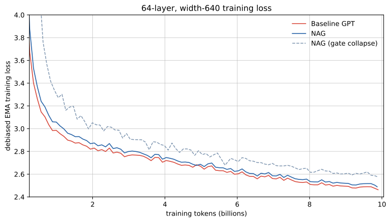Model Config:

Setting	Shared configuration
Architecture	64 Transformer blocks, model dimension 640
Attention	5 heads × 128 head dimension; full-context attention in every layer
Sequence length	2,048 tokens
Vocabulary	32,768 tokens (nanochat tokenizer)
Embeddings	Untied input and output embeddings
Precision	bf16 compute with fp32 master weights; NAG norm lane $s_l$ kept in fp32
GPT parameters	≈356.5M total: 314.6M matrix parameters + 2 × 21.0M embedding parameters
NAG parameters	GPT parameters + ≈2.6M gate parameters (`m_down` 640→32 per sublayer, coefficients, $\beta$, and $\alpha$), a 0.7% increase
Data	Same climbmix shards and tokenizer for both runs

Train Config:

Setting	GPT	NAG
Hardware	8 × H100	8 × H100
Compute budget	$3 × 10^{19}$ FLOPs	$3 × 10^{19}$ FLOPs
Training length	9,474 steps / 9.93B tokens	9,425 steps / 9.88B tokens
Batch size	1,048,576 tokens (device batch 16 + gradient accumulation)	Same
Schedule	40-step LR warmup; linear warmdown over the final 65% to 5%	Same
Matrix optimizer	Muon: LR 0.012, momentum 0.95	Same
Other optimizer	AdamW: embedding LR 0.18, unembedding LR 0.006, temperature-gain LR 0.005	Same, plus gate and $\alpha$ LR of $10^{-3}$
Batch scaling	All learning rates ×$\sqrt{2}$ for a $2^{20}$-token batch vs. the $2^{19}$ reference	Same
NAG initialization and warmup	—	Residual-update injection ramped over the first 314.6M tokens (~300 steps); $C=32$; $\beta=0.5413=\operatorname{softplus}^{-1}(1)$; $\alpha=1/\sqrt{\text{update index}}$; gate bias 0
Architecture details	Pre-norm, QK-norm ×1.2, ReLU² MLP, logit softcap 15, zero-initialized projections	Same attention/MLP internals; cosine decoding ×$e^{s_L}$; no softcap

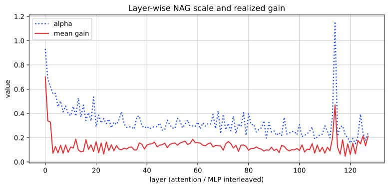
My experiments reproduced the paper's main geometric findings pretty well. Let's walk through the key claims. First, does a plain transformer's residual norm really blow up with depth, and does NAG rein it in? The first panel compares residual-stream norm through depth, with the baseline GPT’s norm growing dramatically, while NAG keeps it controlled. The baseline’s final norm spike is caused by the BOS token becoming an outlier. The second panel shows cumulative residual rotation. NAG accumulates rotation more consistently through depth (closely resembling the paper’s Figure 3c). NAG's rotation accumulates at a steady, near-linear rate, meaning each layer contributes a roughly equal share of the total rotation. In contrast, the baseline cumulative rotation is flatter until making one final massive write before decoding, producing a $\sim60^\circ$ rotation (probably a last-minute correction to set up the output logits, since there's no downstream layer whose representation it needs to preserve). 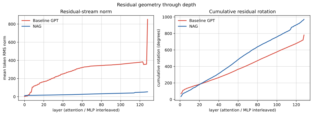Zooming in on NAG's sublayers, they also have fairly uniform realized gain on average. The learned $\alpha_l$ values and mean gains follow the same broad layerwise pattern as the paper’s Figure 5. Their values are generally lower here, likely because my model has twice as many residual updates and initializes $\alpha_l$ as $1/\sqrt{\text{update index}}$. For the attention sink, my NAG model didn’t eliminate the BOS attention sink, but it reduced reliance on it, lowering mean attention assigned to BOS by 26% relative. The distribution of layers using the sink also shifted substantially compared to the baseline. In the baseline GPT 59 of 64 layers assigned more than 50% of their attention to the first (BOS) key, while only 27 of 64 layers did so in NAG. Interestingly, in NAG, the sink influence grew through depth, with attention increasing approximately 32.6%, 39.2%, 53.5%, and 60.8% across the four depth quartiles.

Metric	GPT baseline	NAG
Mean attention assigned to BOS/key 0	62.5%	46.5%
Mean attention assigned to first four keys	65.3%	50.9%
Mean diagonal/self-attention	5.2%	6.7%

Finally, can residual norm serve as a useful confidence signal? The first panel shows the expected mechanical relationship: because norm scales the logits, entropy generally falls as norm increases. More interestingly, the other two panels show that tokens with larger residual norms also have lower next-token loss and higher top-1 accuracy. The dashed curve ranks the same tokens by output entropy, which is the conventional post-hoc confidence measure any language model has, computed from the final probability distribution. The baseline and NAG have similar output entropy, but NAG exposes a dedicated scalar confidence signal before the output projection and allows us to track how that signal develops through depth. 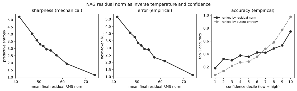This is also my best guess for why NAG won CORE despite losing on raw loss. CORE largely selects among candidate completions using their mean token loss, and NAG’s token-dependent logit scale could improve those rankings even while average compression remains slightly worse.

NAG Update

The NAG update is fairly compact, but three practical details are worth highlighting. First, the weighted sigmoid sum is clamped to $10^{-6}$ before applying the exponent, preventing the infinite gradient described above. Second, $\beta_l$ is passed through `softplus` to keep it positive, ensuring the modulator remains between zero and one. Finally, I RMS-normalize the updated direction directly instead of dividing by $\sqrt{1 + \alpha_l^2 m_l^2(\bar{R}_l)}$; in bf16, measuring the norm prevents small numerical errors from accumulating and pulling the direction stream away from its hypersphere. Here, `branch_out` is the raw attention or MLP output. ```python class NAGResBranch(nn.Module): def __init__(self, config): super().__init__() C = 32 self.m_down = Linear(config.n_embd, C, bias=True) self.coef = nn.Parameter(torch.zeros(C)) self.beta = nn.Parameter(torch.zeros(1))

self.alpha = nn.Parameter(torch.zeros(1)) self.register_buffer( "alpha_warmup_scale", torch.ones(()), persistent=False )

def forward(self, res_log_norm, res_dir, branch_out): u = ( F.softmax(self.coef, dim=0) * F.sigmoid(self.m_down(res_dir)) ).sum(dim=-1) beta = F.softplus(self.beta)

clamp to avoid inf backward gradient when u = 0

modulator = u.clamp_min(1e-6).pow(beta).unsqueeze(-1)

branch_scale = modulator self.alpha self.alpha_warmup_scale branch_scale_sq = branch_scale.square()

centered_x = branch_out - branch_out.mean(dim=-1, keepdim=True) parallel_x = res_dir ( (centered_x res_dir).sum(dim=-1, keepdim=True) / res_dir.square().sum(dim=-1, keepdim=True) ) orth_x = centered_x - parallel_x orth_x = norm(orth_x)

switched to pure rms norm as dividing by predicted norm gain causes compounding res_dir drift due to precision

res_dir = (

res_dir + branch_scale.to(res_dir.dtype) * orth_x

) / torch.sqrt(1 + branch_scale_sq).to(res_dir.dtype)

res_dir = norm(res_dir + branch_scale.to(res_dir.dtype) orth_x) res_log_norm = res_log_norm + torch.log1p(branch_scale_sq) 0.5

return res_log_norm, res_dir ```

Conclusion

My experiments did not reproduce a clean loss improvement. The baseline finished with lower training loss and validation bpb, while NAG performed better on CORE. Still, my NAG implementation reproduced the paper’s main geometric findings: controlled residual-norm growth, steadier rotation through depth, and less reliance on the BOS attention sink. Given that I used a different, dense architecture and trained for far fewer tokens, I see these results as encouraging rather than conclusive.

The failed runs provided some good lessons in their own right. The one I keep thinking about is the gate collapse: tiny, poorly learned early outputs get normalized straight to full size, so the modulator learns to shut those layers off and, starved of gradient, they never recover. The geometry was not fundamentally broken, but the training setup needed more care. I should have run a few tiny experiments and checked whether the loss and gate values behaved as expected before launching the full run. Catching this earlier would have saved me time. Lowering the modulator’s learning rate and gradually warming up $\alpha_l$ were enough to keep the gates alive. Architectures are often judged less by their underlying merits than by whether they survive a real training loop. Most of that diagnosis happened on two consumer GPUs at roughly 75 minutes a run, before I ever touched an H100. So you do not always need a cluster to do real architecture science; sometimes you only need one to confirm the final result at scale.

I really enjoyed working through this paper because it takes one of the most familiar components in deep learning, the residual stream, and asks whether we have been using it in the best way. NAG’s central idea is simple: separate direction from magnitude, let each layer control how much it rotates the residual, and track the resulting norm explicitly. From that one geometric change, the paper gets better depth utilization, a per-token scalar that can be interpreted as confidence, and a natural route toward adaptive-depth computation.

What I would do next:

- Write fused kernels. In an earlier measurement, the unfused implementation was roughly 40% slower and used 24% more memory than the baseline GPT. - Implement MoD for both inference and training. - Try the direction-and-magnitude split on recurrent models like TRM and EqR, where keeping a repeatedly reused state stable makes the same separation especially interesting.

References

- Scaling Adaptive Depth with Norm-Agnostic Residual Networks - NAG-nanochat repo - original nanochat repo - nGPT: Normalized Transformer with Representation Learning on the Hypersphere - Tapered Language Models - MoLAE: Mixture of Latent Experts for Parameter-Efficient Language Models - Compressed Convolutional Attention: Efficient Attention in a Compressed Latent Space - Mixture-of-Depths: Dynamically allocating compute in transformer-based language models - Less is More: Recursive Reasoning with Tiny Networks - Equilibrium Reasoners: Learning Attractors Enables Scalable Reasoning